PySpark is an API of Apache Spark which is an open-source, distributed processing system used for big data processing which was originally developed in Scala programming language at UC Berkely. Spark has development APIs in Scala, Java, Python, and R, and supports code reuse across multiple workloads — batch processing, interactive queries, real-time analytics, machine learning, and graph processing. It utilizes in-memory caching, and optimized query execution for fast analytic queries against data of any size. It does not have its own file system like Hadoop HDFS, it supports most of all popular file systems like Hadoop Distributed File System (HDFS), HBase, Cassandra, Amazon S3, Amazon Redshift, Couchbase, e.t.c.
The Advantages of using Apache Spark:
- It runs programs up to 100x faster than Hadoop MapReduce in memory, or 10x faster on disk. It claims because it does the processing in the main memory of the worker nodes and prevents unnecessary I/O operations.
- It is user-friendly as it has APIs written in popular languages which makes it easy for your developers because they hide the complexity of distributed processing behind simple, high-level operators that dramatically lowers the amount of code required.
- It Can be deployed through Mesos, Hadoop via Yarn, or Spark’s own cluster manager.
- Real-time computation and low latency because of in-memory computation.
In this article, we try to understand the below concepts:
- Setting Environment in Google Colab
- Spark Session
- Reading Data
- Structuring Data Using Spark Schema
- Different Methods to Inspect Data
- Column Manipulation
- Dealing with Missing Values
- Querying Data
- Data Visualization
- Write/Save Data to File
- Conclusion
Setting Environment in Google Colab
To run pyspark on a local machine we need Java and other software. So instead of the heavy installation procedure, we use Google Colaboratory which has better hardware specifications and also comes with a wide range of libraries for Data Science and Machine Learning. We need to install pyspark and Py4J packages. The Py4J enables Python programs running in a python interpreter to dynamically access Java objects in a Java Virtual Machine. The command to install the above-said packages is
!pip install pyspark==3.0.1 py4j==0.10.9
Spark Session
SparkSession has become an entry point to PySpark since version 2.0 earlier the SparkContext is used as an entry point. The SparkSession is an entry point to underlying PySpark functionality to programmatically create PySpark RDD, DataFrame, and Dataset. It can be used in replace with SQLContext, HiveContext, and other contexts defined before 2.0. You should also know that SparkSession internally creates SparkConfig and SparkContext with the configuration provided with SparkSession. SparkSession can be created using SparkSession.builder builder patterns.
Creating SparkSession
To create a SparkSession, you need to use the builder pattern method builder()
getOrCreate()— the method returns an already existing SparkSession; if not exists, it creates a new SparkSession.master()– If you are running it on the cluster you need to use your master name as an argument. usually, it would be eitheryarnormesosdepends on your cluster setup and also useslocal[X]when running in Standalone mode.Xshould be an integer value and should be greater than 0 which represents how many partitions it should create when using RDD, DataFrame, and Dataset. Ideally, the valueXshould be the number of CPU cores.appName()the method is used to set the name of your application.getOrCreate()the method returns an existing SparkSession if it exists otherwise it creates a new SparkSession.
from pyspark.sql import SparkSession
spark = SparkSession.builder\
        .master("local[*]")\
        .appName('PySpark_Tutorial')\
        .getOrCreate()
# where the '*' represents all the cores of the CPU.
Reading Data
The pyspark can read data from various file formats such as Comma Separated Values (CSV), JavaScript Object Notation (JSON), Parquet, e.t.c. To read different file formats we use spark.read. Here are the examples to read data from different file formats:
# Reading CSV file
csv_file = 'data/stocks_price_final.csv'
df = spark.read.csv(csv_file)
# Reading JSON file
json_file = 'data/stocks_price_final.json'
data = spark.read.json(json_file)
# Reading parquet file
parquet_file = 'data/stocks_price_final.parquet'
data1 = spark.read.parquet(parquet_file)
Structuring Data Using Spark Schema
Let’s read the U.S Stock Price data from January 2019 to July 2020 which is available in Kaggle datasets.
# Before structuring schema
data = spark.read.csv(
    'data/stocks_price_final.csv',
    sep = ',',
    header = True,
    )
data.printSchema()
Let’s see the schema of the data using PrintSchemamethod.
 Spark schema is the structure of the DataFrame or Dataset, we can define it using StructType class which is a collection of StructField that defines the column name(String), column type (DataType), nullable column (Boolean), and metadata (MetaData). spark infers the schema from data however some times the inferred datatype may not be correct or we may need to define our own column names and data types, especially while working with unstructured and semi-structured data.
Let’s see how we can use this to structure our data:
from pyspark.sql.types import *
data_schema = [
               StructField('_c0', IntegerType(), True),
               StructField('symbol', StringType(), True),
               StructField('data', DateType(), True),
               StructField('open', DoubleType(), True),
               StructField('high', DoubleType(), True),
               StructField('low', DoubleType(), True),
               StructField('close', DoubleType(), True),
               StructField('volume', IntegerType(), True),
               StructField('adjusted', DoubleType(), True),
               StructField('market.cap', StringType(), True),
               StructField('sector', StringType(), True),
               StructField('industry', StringType(), True),
               StructField('exchange', StringType(), True),
            ]
final_struc = StructType(fields = data_schema)
data = spark.read.csv(
    'data/stocks_price_final.csv',
    sep = ',',
    header = True,
    schema = final_struc
    )
data.printSchema()
The above code shows how to create structure using StructTypeand StructField. Then pass the created structure to the schema parameter while reading the data using spark.read.csv() . Let’s see the schema of the structured data:
 Different Methods to Inspect Data
There are various methods used to inspect the data. They are schema, dtypes, show, head, first, take, describe, columns, count, distinct, printSchema. Let’s see the explanation of their methods with an example.
- schema(): This method returns the schema of the data(dataframe). The below example w.r.t US StockPrice data is shown.
data.schema

# -------------- Ouput ------------------
# StructType(
#           List(
#             StructField(_c0,IntegerType,true),
#             StructField(symbol,StringType,true),
#             StructField(data,DateType,true),
#             StructField(open,DoubleType,true),
#             StructField(high,DoubleType,true),
#             StructField(low,DoubleType,true),
#             StructField(close,DoubleType,true),
#             StructField(volume,IntegerType,true),
#             StructField(adjusted,DoubleType,true),
#             StructField(market_cap,StringType,true),
#             StructField(sector,StringType,true),
#             StructField(industry,StringType,true),
#             StructField(exchange,StringType,true)
#           )
#         )
- dtypes: It returns a list of tuples with column names and it’s data types.
data.dtypes

#------------- OUTPUT ------------
# [('_c0', 'int'),
#  ('symbol', 'string'),
#  ('data', 'date'),
#  ('open', 'double'),
#  ('high', 'double'),
#  ('low', 'double'),
#  ('close', 'double'),
#  ('volume', 'int'),
#  ('adjusted', 'double'),
#  ('market_cap', 'string'),
#  ('sector', 'string'),
#  ('industry', 'string'),
#  ('exchange', 'string')]
- head(n): It returns n rows as a list. Here is an example:
data.head(3)

# ---------- OUTPUT ---------
# [
#  Row(_c0=1, symbol='TXG', data=datetime.date(2019, 9, 12), open=54.0, high=58.0, low=51.0, close=52.75, volume=7326300, adjusted=52.75, market_cap='$9.31B', sector='Capital Goods', industry='Biotechnology: Laboratory Analytical Instruments', exchange='NASDAQ'),
#  Row(_c0=2, symbol='TXG', data=datetime.date(2019, 9, 13), open=52.75, high=54.355, low=49.150002, close=52.27, volume=1025200, adjusted=52.27, market_cap='$9.31B', sector='Capital Goods', industry='Biotechnology: Laboratory Analytical Instruments', exchange='NASDAQ'),
#  Row(_c0=3, symbol='TXG', data=datetime.date(2019, 9, 16), open=52.450001, high=56.0, low=52.009998, close=55.200001, volume=269900, adjusted=55.200001, market_cap='$9.31B', sector='Capital Goods', industry='Biotechnology: Laboratory Analytical Instruments', exchange='NASDAQ')
# ]
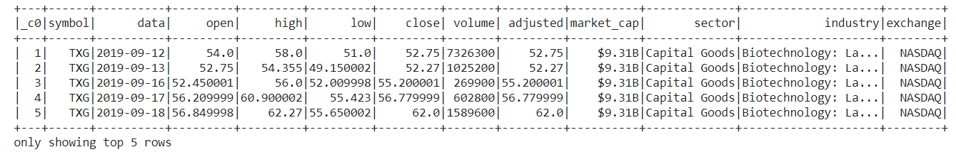
- show(): It displays the first 20 rows by default and it also takes a number as a parameter to display the number of rows of the data. Here is an example: show(5).

- first(): It returns the first row of the data.
data.first()

# ----------- OUTPUT -------------
# Row(_c0=1, symbol='TXG', data=datetime.date(2019, 9, 12), open=54.0, high=58.0, low=51.0, close=52.75, volume=7326300, adjusted=52.75, market_cap='$9.31B', sector='Capital Goods', industry='Biotechnology: Laboratory Analytical Instruments', exchange='NASDAQ')- take(n): It returns the first n rows of the data.
- describe(): It computes the summary statistics of the columns with the numeric data type.
data.describe().show()

# ------------- Output ---------
# +-------+-----------------+-------+------------------+------------------+------------------+------------------+------------------+------------------+----------+----------------+--------------------+--------+
# |summary|              _c0| symbol|              open|              high|               low|             close|            volume|          adjusted|market_cap|          sector|            industry|exchange|
# +-------+-----------------+-------+------------------+------------------+------------------+------------------+------------------+------------------+----------+----------------+--------------------+--------+
# |  count|          1729034|1729034|           1726301|           1726301|           1726301|           1726301|           1725207|           1726301|   1729034|         1729034|             1729034| 1729034|
# |   mean|         864517.5|   null|15070.071703341051| 15555.06726813709|14557.808227578982|15032.714854330707|1397692.1627885813|  14926.1096887955|      null|            null|                null|    null|
# | stddev|499129.2670065541|   null|1111821.8002863196|1148247.1953514954|1072968.1558434265|1109755.9294000647| 5187522.908169119|1101877.6328940107|      null|            null|                null|    null|
# |    min|                1|      A|             0.072|             0.078|             0.052|             0.071|                 0|         -1.230099|    $1.01B|Basic Industries|Accident &Health ...|  NASDAQ|
# |    max|          1729034|   ZYXI|      1.60168176E8|      1.61601456E8|      1.55151728E8|      1.58376592E8|         656504200|      1.57249392E8|       $9B|  Transportation|Wholesale Distrib...|    NYSE|
# +-------+-----------------+-------+------------------+------------------+------------------+------------------+------------------+------------------+----------+----------------+--------------------+--------+
- columns: It returns a list that contains the column names of the data.
data.columns

# --------------- Output --------------
# ['_c0',
#  'symbol',
#  'data',
#  'open',
#  'high',
#  'low',
#  'close',
#  'volume',
#  'adjusted',
#  'market_cap',
#  'sector',
#  'industry',
#  'exchange']
- count(): It returns the count of the number of rows in the data.
data.count()

# returns count of the rows of the data
# -------- output ---------
# 1729034
- distinct(): It returns the number of distinct rows in the data.
- printSchema(): It displays the schema of the data.
df.printSchema()

# ------------ output ------------
# root
#  |-- _c0: integer (nullable = true)
#  |-- symbol: string (nullable = true)
#  |-- data: date (nullable = true)
#  |-- open: double (nullable = true)
#  |-- high: double (nullable = true)
#  |-- low: double (nullable = true)
#  |-- close: double (nullable = true)
#  |-- volume: integer (nullable = true)
#  |-- adjusted: double (nullable = true)
#  |-- market_cap: string (nullable = true)
#  |-- sector: string (nullable = true)
#  |-- industry: string (nullable = true)
#  |-- exchange: string (nullable = true)
Columns Manipulation
Let’s see different methods that are used to add, update, delete columns of the data.
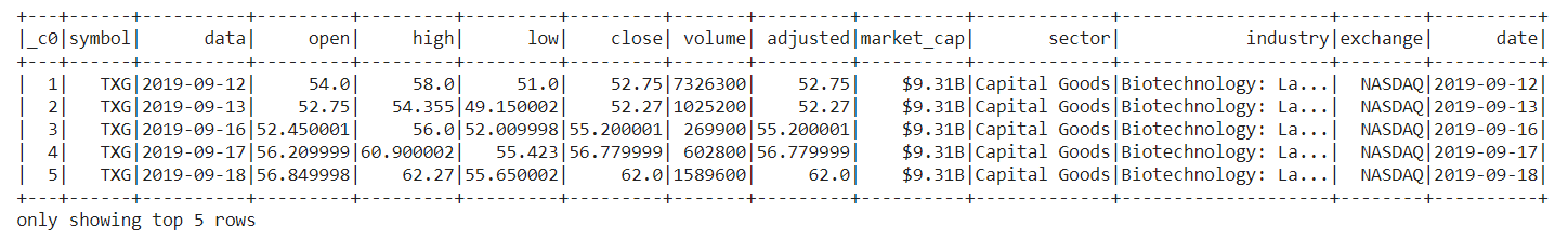
Adding Column: Use withColumn the method takes two parameters column name and data to add a new column to the existing data. See the below example:
data = data.withColumn('date', data.data)
data.show(5)
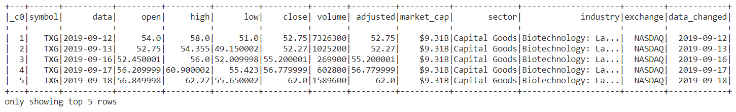
 Update column: Use
 withColumnRenamed which takes to parameters existing column name and new column name to rename the existing column. See the below example:data = data.withColumnRenamed('date', 'data_changed')
data.show(5)
Delete Column: Use drop the method which takes the column name and returns the data.
data = data.drop('data_changed')
data.show(5)
Dealing with Missing Values
We often encounter missing values while dealing with real-time data. These missing values are encoded as NaN, Blanks, and placeholders. There are various techniques to deal with missing values some of the popular ones are:
- Remove: Remove the rows having missing values in any one of the columns.
- Impute with Mean/Median: Replace the missing values using the Mean/Median of the respective column. It’s easy, fast, and works well with small numeric datasets.
- Impute with Most Frequent Values: As the name suggests use the most frequent value in the column to replace the missing value of that column. This works well with categorical features and may also introduce bias into the data.
- Impute using KNN: K-Nearest Neighbors is a classification algorithm that uses feature similarity using different distance metrics such as Euclidean, Mahalanobis, Manhattan, Minkowski, and Hamming e.t.c. for any new data points. This is very efficient compared to the above-mentioned methods to impute missing values depending on the dataset and it is computationally expensive and sensitive to outliers.
Let’s see how we can use PySpark to deal with missing values:
# Remove Rows with Missing Values
data.na.drop()
# Replacing Missing Values with Mean
data.na.fill(data.select(f.mean(data['open'])).collect()[0][0])
# Replacing Missing Values with new values
data.na.replace(old_value, new_vallue)
Querying Data
The PySpark and PySpark SQL provide a wide range of methods and functions to query the data at ease. Here are the few most used methods:
- Select
- Filter
- Between
- When
- Like
- GroupBy
- Aggregations
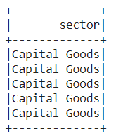
Select
It is used to select single or multiple columns using the names of the columns. Here is a simple example:
## Selecting Single Column
data.select('sector').show(5)
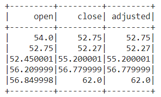
## Selecting Multiple columns
data.select(['open', 'close', 'adjusted']).show(5)
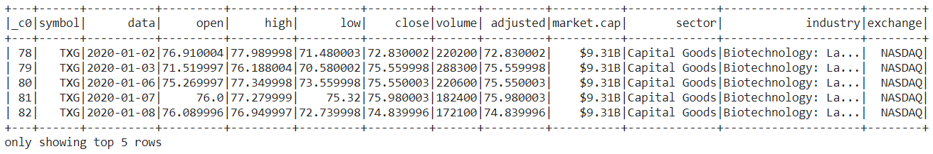
Filter
Filter the data based on the given condition, you can also give multiple conditions using AND(&), OR(|), and NOT(~) operators. Here is the example to fetch the data of January 2020 stock prices.
from pyspark.sql.functions import col, lit
data.filter( (col('data') >= lit('2020-01-01')) & (col('data') <= lit('2020-01-31')) ).show(5)
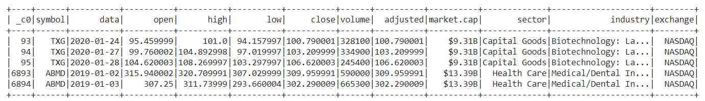
Between
This method returns either True or False if the passed values in the between method. Let’s see an example to fetch the data where the adjusted value is between 100 and 500.
## fetch the data where the adjusted value is between 100.0 and 500.0
data.filter(data.adjusted.between(100.0, 500.0)).show()
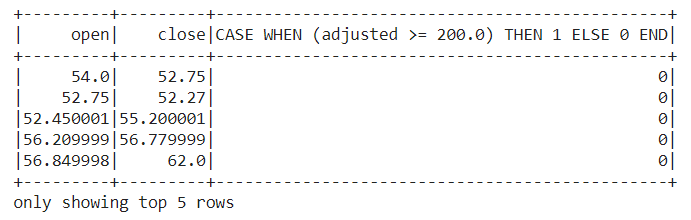
When
It returns 0 or 1 depending on the given condition, the below example shows how to select the opening and closing price of stocks when the adjusted price is greater than equals to 200.
data.select('open', 'close',
            f.when(data.adjusted >= 200.0, 1).otherwise(0)
           ).show(5)
Like
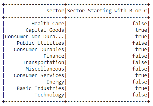
It is similar to the like operator in SQL, The below example show to extract the sector names which stars with either M or C using ‘rlike’.
data.select('sector',
            data.sector.rlike('^[B,C]').alias('Sector Starting with B or C')
            ).distinct().show()
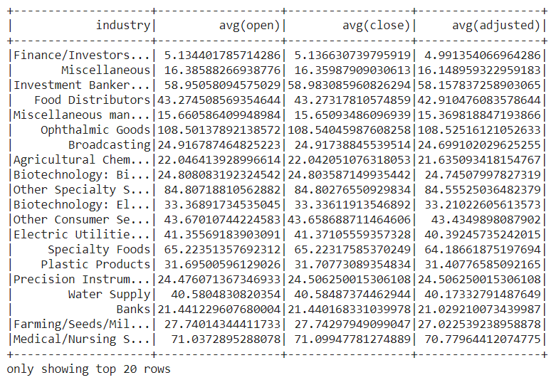
GourpBy
The name itself explains that it groups the data by the given column name and it can perform different operations such as sum, mean, min, max, e.t.c. The below example explains how to get the average opening, closing, and adjusted stock price concerning industries.
data.select([
             'industry',
             'open',
             'close',
             'adjusted'
            ]
            ).groupBy('industry')\
            .mean()\
            .show()
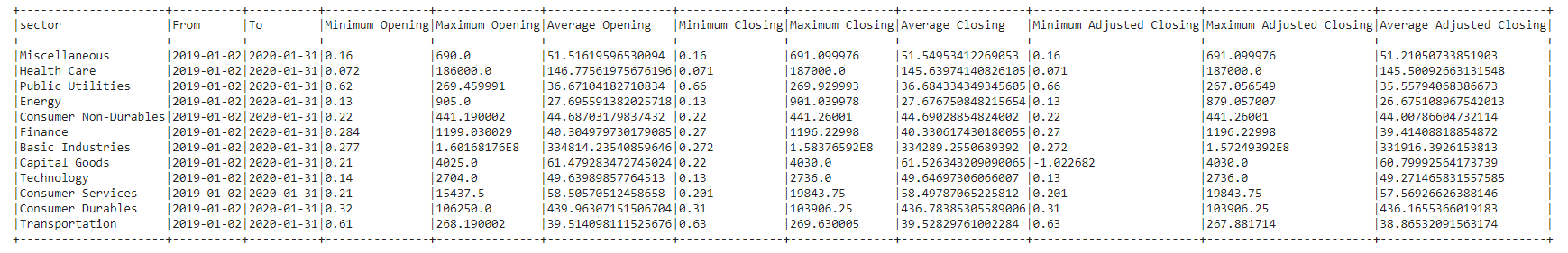
Aggregation
PySpark provides built-in standard Aggregate functions defines in DataFrame API, these come in handy when we need to make aggregate operations on columns of the data. Aggregate functions operate on a group of rows and calculate a single return value for every group. The below example shows how to display the minimum, maximum, and average; opening, closing, and adjusted stock prices from January 2019 to January 2020 concerning the sectors.
data.filter( (col('data') >= lit('2019-01-02')) & (col('data') <= lit('2020-01-31')) )\
    .groupBy("sector") \
    .agg(min("data").alias("From"),
         max("data").alias("To"),

         min("open").alias("Minimum Opening"),
         max("open").alias("Maximum Opening"),
         avg("open").alias("Average Opening"),

         min("close").alias("Minimum Closing"),
         max("close").alias("Maximum Closing"),
         avg("close").alias("Average Closing"),

         min("adjusted").alias("Minimum Adjusted Closing"),
         max("adjusted").alias("Maximum Adjusted Closing"),
         avg("adjusted").alias("Average Adjusted Closing"),

      ).show(truncate=False)
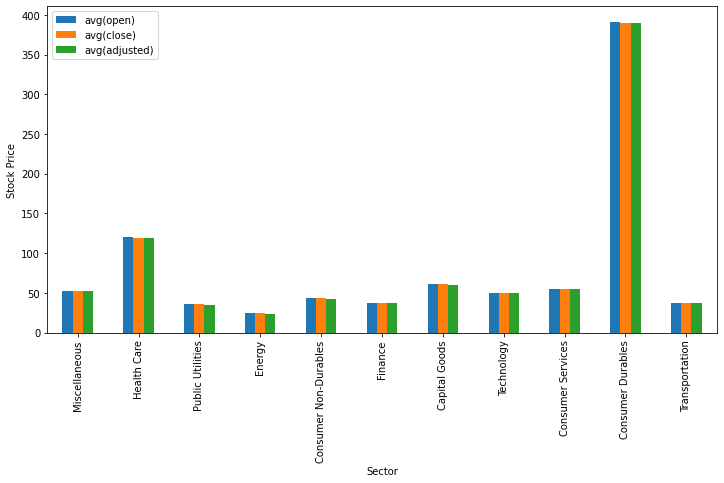
Data Visualization
We are going to utilize matplotlib and pandas to visualize data, the toPandas() method used to convert the data into pandas dataframe. Using the dataframe we utilize the plot() method to visualize data. The below code shows how to display a bar graph for the average opening, closing, and adjusted stock price concerning the sector.
sec_df =  data.select(['sector',
                       'open',
                       'close',
                       'adjusted']
                     )\
                     .groupBy('sector')\
                     .mean()\
                     .toPandas()

ind = list(range(12))

ind.pop(6)

sec_df.iloc[ind ,:].plot(kind = 'bar', x='sector', y = sec_df.columns.tolist()[1:],
                         figsize=(12, 6), ylabel = 'Stock Price', xlabel = 'Sector')
plt.show()
Similarly, let’s visualize the average opening, closing, and adjusted price concerning industries.
industries_x = data.select(['industry', 'open', 'close', 'adjusted']).groupBy('industry').mean().toPandas()

q  = industries_x[(industries_x.industry != 'Major Chemicals') & (industries_x.industry != 'Building Products')]

q.plot(kind = 'barh', x='industry', y = q.columns.tolist()[1:], figsize=(10, 50), xlabel='Stock Price', ylabel = 'Industry')

plt.show()

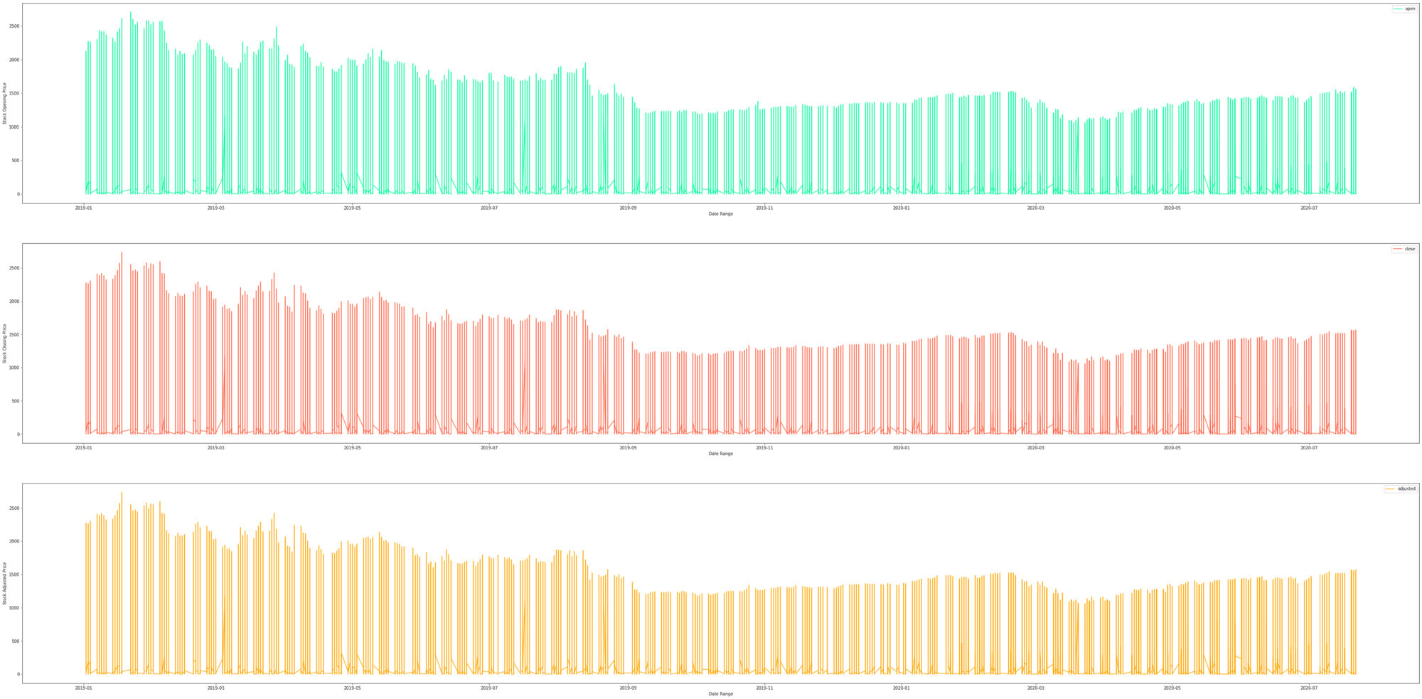
Let’s see the time-series graph of the technology sector average opening, closing, and Adjusted stock price.
from pyspark.sql.functions import col

tech = data.where(col('sector') == 'Technology')\
           .select('data', 'open', 'close', 'adjusted')

fig, axes = plt.subplots(nrows=3, ncols=1, figsize =(60, 30))

tech.toPandas().plot(kind = 'line', x = 'data', y='open',
                     xlabel = 'Date Range', ylabel = 'Stock Opening Price',
                     ax = axes[0], color = 'mediumspringgreen')

tech.toPandas().plot(kind = 'line', x = 'data', y='close',
                     xlabel = 'Date Range', ylabel = 'Stock Closing Price',
                     ax = axes[1], color = 'tomato')

tech.toPandas().plot(kind = 'line', x = 'data', y='adjusted',
                     xlabel = 'Date Range', ylabel = 'Stock Adjusted Price',
                     ax = axes[2], color = 'orange')

plt.show()
Write/Save Data to File
The ‘write.save()’ method is used to save the data in different formats such as CSV, JSVON, Parquet, e.t.c. Let’s see how to save the data in different file formats. We can able to save entire data and selected data using the ‘select()’ method.
## Writing entire data to different file formats

# CSV
data.write.csv('dataset.csv')

# JSON
data.write.save('dataset.json', format='json')

# Parquet
data.write.save('dataset.parquet', format='parquet')

## Writing selected data to different file formats

# CSV
data.select(['data', 'open', 'close', 'adjusted'])\
            .write.csv('dataset.csv')

# JSON
data.select(['data', 'open', 'close', 'adjusted'])\
    .write.save('dataset.json', format='json')

# Parquet
data.select(['data', 'open', 'close', 'adjusted'])\
    .write.save('dataset.parquet', format='parquet')
Conclusion
PySpark is a great language for data scientists to learn because it enables scalable analysis and ML pipelines. If you’re already familiar with Python and SQL and Pandas, then PySpark is a great way to start.
This article showed how to perform a wide range of operations starting with reading files to writing insights to file using PySpark. It’s also covered the basic visualization techniques using matplotlib to visualize the insights. Moreover, Google Colaboratory Notebooks is a great way to start learning PySpark without installing the necessary software. C