PySpark Tutorial for Beginners

What is Apache Spark?

Spark is a big data solution that has been proven to be easier and faster than Hadoop MapReduce. Spark is an open source software developed by UC Berkeley RAD lab in 2009. Since it was released to the public in 2010, Spark has grown in popularity and is used through the industry with an unprecedented scale.

In the era of Big Data, practitioners need more than ever fast and reliable tools to process streaming of data. Earlier tools like MapReduce were favorite but were slow. To overcome this issue, Spark offers a solution that is both fast and general-purpose. The main difference between Spark and MapReduce is that Spark runs computations in memory during the later on the hard disk. It allows high-speed access and data processing, reducing times from hours to minutes.

In this PySpark tutorial for beginners, you will learn PySpark basics like-

• How Does Spark work?
• Why use Spark?
• How to Install Pyspark with AWS
• How to Install PySpark on Windows/Mac with Conda
• Spark Context
• SQLContext
• Machine Learning Example with PySpark
• Step 1) Basic operation with PySpark
• Step 2) Data preprocessing
• Step 3) Build a data processing pipeline
• Step 4) Build the classifier: logistic
• Step 5) Train and evaluate the model
• Step 6) Tune the hyperparameter

How Does Spark work?

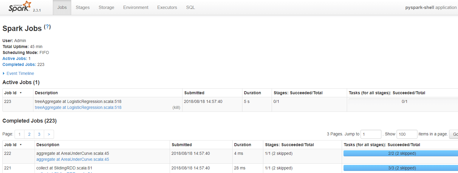
Spark is based on computational engine, meaning it takes care of the scheduling, distributing and monitoring application. Each task is done across various worker machines called computing cluster. A computing cluster refers to the division of tasks. One machine performs one task, while the others contribute to the final output through a different task. In the end, all the tasks are aggregated to produce an output. The Spark admin gives a 360 overview of various Spark Jobs.

How does Spark Work

Spark is designed to work with

• Python
• Java
• Scala
• SQL

A significant feature of Spark is the vast amount of built-in library, including MLlib for machine learning. Spark is also designed to work with Hadoop clusters and can read the broad type of files, including Hive data, CSV, JSON, Casandra data among other.

Why use Spark?

As a future data practitioner, you should be familiar with python’s famous libraries: Pandas and scikit-learn. These two libraries are fantastic to explore dataset up to mid-size. Regular machine learning projects are built around the following methodology:

• Load the data to the disk
• Import the data into the machine’s memory
• Process/analyze the data
• Build the machine learning model
• Store the prediction back to disk

The problem arises if the data scientist wants to process data that’s too big for one computer. During earlier days of data science, the practitioners would sample the as training on huge data sets was not always needed. The data scientist would find a good statistical sample, perform an additional robustness check and comes up with an excellent model.

However, there are some problems with this:

• Is the dataset reflecting the real world?
• Does the data include a specific example?
• Is the model fit for sampling?

Take users recommendation for instance. Recommenders rely on comparing users with other users in evaluating their preferences. If the data practitioner takes only a subset of the data, there won’t be a cohort of users who are very similar to one another. Recommenders need to run on the full dataset or not at all.

What is the solution?

The solution has been evident for a long time, split the problem up onto multiple computers. Parallel computing comes with multiple problems as well. Developers often have trouble writing parallel code and end up having to solve a bunch of the complex issues around multi-processing itself.

Pyspark gives the data scientist an API that can be used to solve the parallel data proceedin problems. Pyspark handles the complexities of multiprocessing, such as distributing the data, distributing code and collecting output from the workers on a cluster of machines.

Spark can run standalone but most often runs on top of a cluster computing framework such as Hadoop. In test and development, however, a data scientist can efficiently run Spark on their development boxes or laptops without a cluster

• One of the main advantages of Spark is to build an architecture that encompasses data streaming management, seamlessly data queries, machine learning prediction and real-time access to various analysis.

• Spark works closely with SQL language, i.e., structured data. It allows querying the data in real time.

• Data scientist main’s job is to analyze and build predictive models. In short, a data scientist needs to know how to query data using SQL, produce a statistical report and make use of machine learning to produce predictions. Data scientist spends a significant amount of their time on cleaning, transforming and analyzing the data. Once the dataset or data workflow is ready, the data scientist uses various techniques to discover insights and hidden patterns. The data manipulation should be robust and the same easy to use. Spark is the right tool thanks to its speed and rich APIs.

In this PySpark tutorial, you will learn how to build a classifier with PySpark examples.

sudo yum update -y
sudo yum install -y docker
sudo service docker start
sudo user-mod -a -G docker ec2-user
exit

## Spark
docker run -v ~/work:/home/jovyan/work -d -p 8888:8888 jupyter/pyspark-notebook

## Allow preserving Jupyter notebook
sudo chown 1000 ~/work

## Install tree to see our working directory next
sudo yum install -y tree

docker ps

cd anaconda3
touch hello-spark.yml
vi hello-spark.yml

cd C:\Users\Admin\Anaconda3
echo.>hello-spark.yml
notepad hello-spark.yml

name: hello-spark 
    dependencies:
    
    - python=3.6
    - jupyter
    - ipython
    - numpy
    - numpy-base
    - pandas
    - py4j
    - pyspark
    - pytz

conda env create -f hello-spark.yml

conda env list

Activate hello-spark

source activate hello-spark

activate hello-spark

Imagine most of your project involves TensorFlow, but you need to use Spark for one particular project. You can set a TensorFlow environment for all your project and create a separate environment for Spark. You can add as many libraries in Spark environment as you want without interfering with the TensorFlow environment. Once you are done with the Spark’s project, you can erase it without affecting the TensorFlow environment.

Jupyter

Open Jupyter Notebook and try if PySpark works. In a new notebook paste the following PySpark sample code:

import pyspark
from pyspark import SparkContext
sc =SparkContext()

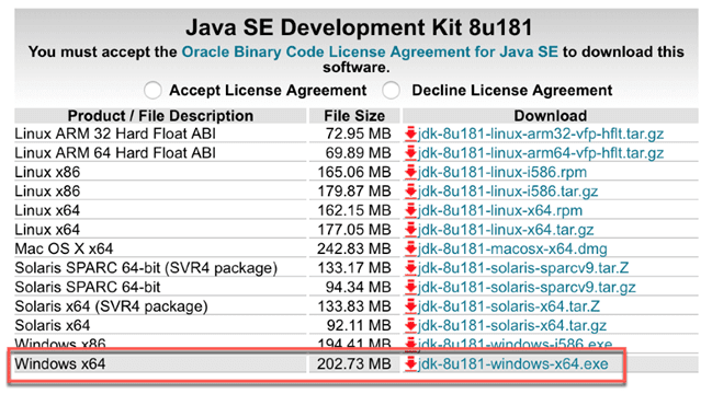
If an error is shown, it is likely that Java is not installed on your machine. In mac, open the terminal and write java -version, if there is a java version, make sure it is 1.8. In Windows, go to Application and check if there is a Java folder. If there is a Java folder, check that Java 1.8 is installed. As of this writing, PySpark is not compatible with Java9 and above.

If you need to install Java, you to think link and download jdk-8u181-windows-x64.exe

For Mac User, it is recommended to use `brew.`

brew tap caskroom/versions
brew cask install java8

 conda env remove -n hello-spark -y

Spark Context

SparkContext is the internal engine that allows the connections with the clusters. If you want to run an operation, you need a SparkContext.

Create a SparkContext

First of all, you need to initiate a SparkContext.

import pyspark
from pyspark import SparkContext
sc =SparkContext()

Now that the SparkContext is ready, you can create a collection of data called RDD, Resilient Distributed Dataset. Computation in an RDD is automatically parallelized across the cluster.

nums= sc.parallelize([1,2,3,4])

You can access the first row with take

nums.take(1)

[1]

You can apply a transformation to the data with a lambda function. In the PySpark example below, you return the square of nums. It is a map transformation

squared = nums.map(lambda x: x*x).collect()
for num in squared:
    print('%i ' % (num))

1 
4 
9 
16

SQLContext

A more convenient way is to use the DataFrame. SparkContext is already set, you can use it to create the dataFrame. You also need to declare the SQLContext

SQLContext allows connecting the engine with different data sources. It is used to initiate the functionalities of Spark SQL.

from pyspark.sql import Row
from pyspark.sql import SQLContext

sqlContext = SQLContext(sc)

Now in this Spark tutorial Python, let’s create a list of tuple. Each tuple will contain the name of the people and their age. Four steps are required:

Step 1) Create the list of tuple with the information

[('John',19),('Smith',29),('Adam',35),('Henry',50)]

Step 2) Build a RDD

rdd = sc.parallelize(list_p)

Step 3) Convert the tuples

rdd.map(lambda x: Row(name=x[0], age=int(x[1])))

Step 4) Create a DataFrame context

sqlContext.createDataFrame(ppl)
list_p = [('John',19),('Smith',29),('Adam',35),('Henry',50)]
rdd = sc.parallelize(list_p)
ppl = rdd.map(lambda x: Row(name=x[0], age=int(x[1])))
DF_ppl = sqlContext.createDataFrame(ppl)

If you want to access the type of each feature, you can use printSchema()

DF_ppl.printSchema()
root
 |-- age: long (nullable = true)
 |-- name: string (nullable = true)

Machine Learning Example with PySpark

Now that you have a brief idea of Spark and SQLContext, you are ready to build your first Machine learning program.

Following are the steps to build a Machine Learning program with PySpark:

• Step 1) Basic operation with PySpark
• Step 2) Data preprocessing
• Step 3) Build a data processing pipeline
• Step 4) Build the classifier: logistic
• Step 5) Train and evaluate the model
• Step 6) Tune the hyperparameter

In this PySpark Machine Learning tutorial, we will use the adult dataset. The purpose of this tutorial is to learn how to use Pyspark. For more information about the dataset, refer to this tutorial.

Note that, the dataset is not significant and you may think that the computation takes a long time. Spark is designed to process a considerable amount of data. Spark’s performances increase relative to other machine learning libraries when the dataset processed grows larger.

Step 1) Basic operation with PySpark

First of all, you need to initialize the SQLContext is not already in initiated yet.

#from pyspark.sql import SQLContext
url = "https://raw.githubusercontent.com/guru99-edu/R-Programming/master/adult_data.csv"
from pyspark import SparkFiles
sc.addFile(url)
sqlContext = SQLContext(sc)

then, you can read the cvs file with sqlContext.read.csv. You use inferSchema set to True to tell Spark to guess automatically the type of data. By default, it is turn to False.

df = sqlContext.read.csv(SparkFiles.get("adult_data.csv"), header=True, inferSchema= True)

Let’s have a look at the data type

df.printSchema()
root
 |-- age: integer (nullable = true)
 |-- workclass: string (nullable = true)
 |-- fnlwgt: integer (nullable = true)
 |-- education: string (nullable = true)
 |-- education_num: integer (nullable = true)
 |-- marital: string (nullable = true)
 |-- occupation: string (nullable = true)
 |-- relationship: string (nullable = true)
 |-- race: string (nullable = true)
 |-- sex: string (nullable = true)
 |-- capital_gain: integer (nullable = true)
 |-- capital_loss: integer (nullable = true)
 |-- hours_week: integer (nullable = true)
 |-- native_country: string (nullable = true)
 |-- label: string (nullable = true)

You can see the data with show.

df.show(5, truncate = False)

+---+----------------+------+---------+-------------+------------------+-----------------+-------------+-----+------+------------+------------+----------+--------------+-----+
|age|workclass       |fnlwgt|education|education_num|marital           |occupation       |relationship |race |sex   |capital_gain|capital_loss|hours_week|native_country|label|
+---+----------------+------+---------+-------------+------------------+-----------------+-------------+-----+------+------------+------------+----------+--------------+-----+
|39 |State-gov       |77516 |Bachelors|13           |Never-married     |Adm-clerical     |Not-in-family|White|Male  |2174        |0           |40        |United-States |<=50K|
|50 |Self-emp-not-inc|83311 |Bachelors|13           |Married-civ-spouse|Exec-managerial  |Husband      |White|Male  |0           |0           |13        |United-States |<=50K|
|38 |Private         |215646|HS-grad  |9            |Divorced          |Handlers-cleaners|Not-in-family|White|Male  |0           |0           |40        |United-States |<=50K|
|53 |Private         |234721|11th     |7            |Married-civ-spouse|Handlers-cleaners|Husband      |Black|Male  |0           |0           |40        |United-States |<=50K|
|28 |Private         |338409|Bachelors|13           |Married-civ-spouse|Prof-specialty   |Wife         |Black|Female|0           |0           |40        |Cuba          |<=50K|
+---+----------------+------+---------+-------------+------------------+-----------------+-------------+-----+------+------------+------------+----------+--------------+-----+
only showing top 5 rows

If you didn’t set inderShema to True, here is what is happening to the type. There are all in string.

df_string = sqlContext.read.csv(SparkFiles.get("adult.csv"), header=True, inferSchema=  False)
df_string.printSchema()
root
 |-- age: string (nullable = true)
 |-- workclass: string (nullable = true)
 |-- fnlwgt: string (nullable = true)
 |-- education: string (nullable = true)
 |-- education_num: string (nullable = true)
 |-- marital: string (nullable = true)
 |-- occupation: string (nullable = true)
 |-- relationship: string (nullable = true)
 |-- race: string (nullable = true)
 |-- sex: string (nullable = true)
 |-- capital_gain: string (nullable = true)
 |-- capital_loss: string (nullable = true)
 |-- hours_week: string (nullable = true)
 |-- native_country: string (nullable = true)
 |-- label: string (nullable = true)

To convert the continuous variable in the right format, you can use recast the columns. You can use withColumn to tell Spark which column to operate the transformation.

# Import all from `sql.types`
from pyspark.sql.types import *

# Write a custom function to convert the data type of DataFrame columns
def convertColumn(df, names, newType):
    for name in names: 
        df = df.withColumn(name, df[name].cast(newType))
    return df 
# List of continuous features
CONTI_FEATURES  = ['age', 'fnlwgt','capital_gain', 'education_num', 'capital_loss', 'hours_week']
# Convert the type
df_string = convertColumn(df_string, CONTI_FEATURES, FloatType())
# Check the dataset
df_string.printSchema()
root
 |-- age: float (nullable = true)
 |-- workclass: string (nullable = true)
 |-- fnlwgt: float (nullable = true)
 |-- education: string (nullable = true)
 |-- education_num: float (nullable = true)
 |-- marital: string (nullable = true)
 |-- occupation: string (nullable = true)
 |-- relationship: string (nullable = true)
 |-- race: string (nullable = true)
 |-- sex: string (nullable = true)
 |-- capital_gain: float (nullable = true)
 |-- capital_loss: float (nullable = true)
 |-- hours_week: float (nullable = true)
 |-- native_country: string (nullable = true)
 |-- label: string (nullable = true)

from pyspark.ml.feature import StringIndexer
#stringIndexer = StringIndexer(inputCol="label", outputCol="newlabel")
#model = stringIndexer.fit(df)
#df = model.transform(df)
df.printSchema()

Select columns

You can select and show the rows with select and the names of the features. Below, age and fnlwgt are selected.

df.select('age','fnlwgt').show(5)

+---+------+
|age|fnlwgt|
+---+------+
| 39| 77516|
| 50| 83311|
| 38|215646|
| 53|234721|
| 28|338409|
+---+------+
only showing top 5 rows

Count by group

If you want to count the number of occurence by group, you can chain:

• groupBy()
• count()

together. In the PySpark example below, you count the number of rows by the education level.

df.groupBy("education").count().sort("count",ascending=True).show()

+------------+-----+
|   education|count|
+------------+-----+
|   Preschool|   51|
|     1st-4th|  168|
|     5th-6th|  333|
|   Doctorate|  413|
|        12th|  433|
|         9th|  514|
| Prof-school|  576|
|     7th-8th|  646|
|        10th|  933|
|  Assoc-acdm| 1067|
|        11th| 1175|
|   Assoc-voc| 1382|
|     Masters| 1723|
|   Bachelors| 5355|
|Some-college| 7291|
|     HS-grad|10501|
+------------+-----+

Describe the data

To get a summary statistics, of the data, you can use describe(). It will compute the :

• count
• mean
• standarddeviation
• min
• max

df.describe().show()

+-------+------------------+-----------+------------------+------------+-----------------+--------+----------------+------------+------------------+------+------------------+----------------+------------------+--------------+-----+
|summary|               age|  workclass|            fnlwgt|   education|    education_num| marital|      occupation|relationship|              race|   sex|      capital_gain|    capital_loss|        hours_week|native_country|label|
+-------+------------------+-----------+------------------+------------+-----------------+--------+----------------+------------+------------------+------+------------------+----------------+------------------+--------------+-----+
|  count|             32561|      32561|             32561|       32561|            32561|   32561|           32561|       32561|             32561| 32561|             32561|           32561|             32561|         32561|32561|
|   mean| 38.58164675532078|       null|189778.36651208502|        null| 10.0806793403151|    null|            null|        null|              null|  null|1077.6488437087312| 87.303829734959|40.437455852092995|          null| null|
| stddev|13.640432553581356|       null|105549.97769702227|        null|2.572720332067397|    null|            null|        null|              null|  null| 7385.292084840354|402.960218649002|12.347428681731838|          null| null|
|    min|                17|          ?|             12285|        10th|                1|Divorced|               ?|     Husband|Amer-Indian-Eskimo|Female|                 0|               0|                 1|             ?|<=50K|
|    max|                90|Without-pay|           1484705|Some-college|               16| Widowed|Transport-moving|        Wife|             White|  Male|             99999|            4356|                99|    Yugoslavia| >50K|
+-------+------------------+-----------+------------------+------------+-----------------+--------+----------------+------------+------------------+------+------------------+----------------+------------------+--------------+-----+

If you want the summary statistic of only one column, add the name of the column inside describe()

df.describe('capital_gain').show()

+-------+------------------+
|summary|      capital_gain|
+-------+------------------+
|  count|             32561|
|   mean|1077.6488437087312|
| stddev| 7385.292084840354|
|    min|                 0|
|    max|             99999|
+-------+------------------+

Crosstab computation

In some occasion, it can be interesting to see the descriptive statistics between two pairwise columns. For instance, you can count the number of people with income below or above 50k by education level. This operation is called a crosstab.

df.crosstab('age', 'label').sort("age_label").show()

+---------+-----+----+
|age_label|<=50K|>50K|
+---------+-----+----+
|       17|  395|   0|
|       18|  550|   0|
|       19|  710|   2|
|       20|  753|   0|
|       21|  717|   3|
|       22|  752|  13|
|       23|  865|  12|
|       24|  767|  31|
|       25|  788|  53|
|       26|  722|  63|
|       27|  754|  81|
|       28|  748| 119|
|       29|  679| 134|
|       30|  690| 171|
|       31|  705| 183|
|       32|  639| 189|
|       33|  684| 191|
|       34|  643| 243|
|       35|  659| 217|
|       36|  635| 263|
+---------+-----+----+
only showing top 20 rows

You can see no people have revenue above 50k when they are young.

Drop column

There are two intuitive API to drop columns:

• drop(): Drop a column
• dropna(): Drop NA’s

Below you drop the column education_num

df.drop('education_num').columns

['age',
 'workclass',
 'fnlwgt',
 'education',
 'marital',
 'occupation',
 'relationship',
 'race',
 'sex',
 'capital_gain',
 'capital_loss',
 'hours_week',
 'native_country',
 'label']

Filter data

You can use filter() to apply descriptive statistics in a subset of data. For instance, you can count the number of people above 40 year old

df.filter(df.age > 40).count()

13443

Descriptive statistics by group

Finally, you can group data by group and compute statistical operations like the mean.

df.groupby('marital').agg({'capital_gain': 'mean'}).show()

+--------------------+------------------+
|             marital| avg(capital_gain)|
+--------------------+------------------+
|           Separated| 535.5687804878049|
|       Never-married|376.58831788823363|
|Married-spouse-ab...| 653.9832535885167|
|            Divorced| 728.4148098131893|
|             Widowed| 571.0715005035247|
|   Married-AF-spouse| 432.6521739130435|
|  Married-civ-spouse|1764.8595085470085|
+--------------------+------------------+

Step 2) Data preprocessing

Data processing is a critical step in machine learning. After you remove garbage data, you get some important insights.

For instance, you know that age is not a linear function with the income. When people are young, their income is usually lower than mid-age. After retirement, a household uses their saving, meaning a decrease in income. To capture this pattern, you can add a square to the age feature

Add age square

To add a new feature, you need to:

1. Select the column
2. Apply the transformation and add it to the DataFrame

from pyspark.sql.functions import *

# 1 Select the column
age_square = df.select(col("age")**2)

# 2 Apply the transformation and add it to the DataFrame
df = df.withColumn("age_square", col("age")**2)

df.printSchema()
root
 |-- age: integer (nullable = true)
 |-- workclass: string (nullable = true)
 |-- fnlwgt: integer (nullable = true)
 |-- education: string (nullable = true)
 |-- education_num: integer (nullable = true)
 |-- marital: string (nullable = true)
 |-- occupation: string (nullable = true)
 |-- relationship: string (nullable = true)
 |-- race: string (nullable = true)
 |-- sex: string (nullable = true)
 |-- capital_gain: integer (nullable = true)
 |-- capital_loss: integer (nullable = true)
 |-- hours_week: integer (nullable = true)
 |-- native_country: string (nullable = true)
 |-- label: string (nullable = true)
 |-- age_square: double (nullable = true)

You can see that age_square has been successfully added to the data frame. You can change the order of the variables with select. Below, you bring age_square right after age.

COLUMNS = ['age', 'age_square', 'workclass', 'fnlwgt', 'education', 'education_num', 'marital',
           'occupation', 'relationship', 'race', 'sex', 'capital_gain', 'capital_loss',
           'hours_week', 'native_country', 'label']
df = df.select(COLUMNS)
df.first()

Row(age=39, age_square=1521.0, workclass='State-gov', fnlwgt=77516, education='Bachelors', education_num=13, marital='Never-married', occupation='Adm-clerical', relationship='Not-in-family', race='White', sex='Male', capital_gain=2174, capital_loss=0, hours_week=40, native_country='United-States', label='<=50K')

Exclude Holand-Netherlands

When a group within a feature has only one observation, it brings no information to the model. On the contrary, it can lead to an error during the cross-validation.

Let’s check the origin of the household

df.filter(df.native_country == 'Holand-Netherlands').count()
df.groupby('native_country').agg({'native_country': 'count'}).sort(asc("count(native_country)")).show()

+--------------------+---------------------+
|      native_country|count(native_country)|
+--------------------+---------------------+
|  Holand-Netherlands|                    1|
|            Scotland|                   12|
|             Hungary|                   13|
|            Honduras|                   13|
|Outlying-US(Guam-...|                   14|
|          Yugoslavia|                   16|
|            Thailand|                   18|
|                Laos|                   18|
|            Cambodia|                   19|
|     Trinadad&Tobago|                   19|
|                Hong|                   20|
|             Ireland|                   24|
|             Ecuador|                   28|
|              Greece|                   29|
|              France|                   29|
|                Peru|                   31|
|           Nicaragua|                   34|
|            Portugal|                   37|
|                Iran|                   43|
|               Haiti|                   44|
+--------------------+---------------------+
only showing top 20 rows

The feature native_country has only one household coming from Netherland. You exclude it.

df_remove = df.filter(df.native_country !=	'Holand-Netherlands')

Step 3) Build a data processing pipeline

Similar to scikit-learn, Pyspark has a pipeline API.

A pipeline is very convenient to maintain the structure of the data. You push the data into the pipeline. Inside the pipeline, various operations are done, the output is used to feed the algorithm.

For instance, one universal transformation in machine learning consists of converting a string to one hot encoder, i.e., one column by a group. One hot encoder is usually a matrix full of zeroes.

The steps to transform the data are very similar to scikit-learn. You need to:

• Index the string to numeric
• Create the one hot encoder
• Transform the data

Two APIs do the job: StringIndexer, OneHotEncoder

1. First of all, you select the string column to index. The inputCol is the name of the column in the dataset. outputCol is the new name given to the transformed column.

StringIndexer(inputCol="workclass", outputCol="workclass_encoded")

2. Fit the data and transform it

model = stringIndexer.fit(df)		
`indexed = model.transform(df)``

3. Create the news columns based on the group. For instance, if there are 10 groups in the feature, the new matrix will have 10 columns, one for each group.

OneHotEncoder(dropLast=False, inputCol="workclassencoded", outputCol="workclassvec")

### Example encoder
from pyspark.ml.feature import StringIndexer, OneHotEncoder, VectorAssembler

stringIndexer = StringIndexer(inputCol="workclass", outputCol="workclass_encoded")
model = stringIndexer.fit(df)
indexed = model.transform(df)
encoder = OneHotEncoder(dropLast=False, inputCol="workclass_encoded", outputCol="workclass_vec")
encoded = encoder.transform(indexed)
encoded.show(2)

+---+----------+----------------+------+---------+-------------+------------------+---------------+-------------+-----+----+------------+------------+----------+--------------+-----+-----------------+-------------+
|age|age_square|       workclass|fnlwgt|education|education_num|           marital|     occupation| relationship| race| sex|capital_gain|capital_loss|hours_week|native_country|label|workclass_encoded|workclass_vec|
+---+----------+----------------+------+---------+-------------+------------------+---------------+-------------+-----+----+------------+------------+----------+--------------+-----+-----------------+-------------+
| 39|    1521.0|       State-gov| 77516|Bachelors|           13|     Never-married|   Adm-clerical|Not-in-family|White|Male|        2174|           0|        40| United-States|<=50K|              4.0|(9,[4],[1.0])|
| 50|    2500.0|Self-emp-not-inc| 83311|Bachelors|           13|Married-civ-spouse|Exec-managerial|      Husband|White|Male|           0|           0|        13| United-States|<=50K|              1.0|(9,[1],[1.0])|
+---+----------+----------------+------+---------+-------------+------------------+---------------+-------------+-----+----+------------+------------+----------+--------------+-----+-----------------+-------------+
only showing top 2 rows

Build the pipeline

You will build a pipeline to convert all the precise features and add them to the final dataset. The pipeline will have four operations, but feel free to add as many operations as you want.

1. Encode the categorical data
2. Index the label feature
3. Add continuous variable
4. Assemble the steps.

Each step is stored in a list named stages. This list will tell the VectorAssembler what operation to perform inside the pipeline.

1. Encode the categorical data

This step is exaclty the same as the above example, except that you loop over all the categorical features.

from pyspark.ml import Pipeline
from pyspark.ml.feature import OneHotEncoderEstimator
CATE_FEATURES = ['workclass', 'education', 'marital', 'occupation', 'relationship', 'race', 'sex', 'native_country']
stages = [] # stages in our Pipeline
for categoricalCol in CATE_FEATURES:
    stringIndexer = StringIndexer(inputCol=categoricalCol, outputCol=categoricalCol + "Index")
    encoder = OneHotEncoderEstimator(inputCols=[stringIndexer.getOutputCol()],
                                     outputCols=[categoricalCol + "classVec"])
    stages += [stringIndexer, encoder]

2. Index the label feature

Spark, like many other libraries, does not accept string values for the label. You convert the label feature with StringIndexer and add it to the list stages

# Convert label into label indices using the StringIndexer
label_stringIdx =  StringIndexer(inputCol="label", outputCol="newlabel")
stages += [label_stringIdx]

3. Add continuous variable

The inputCols of the VectorAssembler is a list of columns. You can create a new list containing all the new columns. The code below popluate the list with encoded categorical features and the continuous features.

assemblerInputs = [c + "classVec" for c in CATE_FEATURES] + CONTI_FEATURES

4. Assemble the steps.

Finally, you pass all the steps in the VectorAssembler

assembler = VectorAssembler(inputCols=assemblerInputs, outputCol="features")stages += [assembler]

Now that all the steps are ready, you push the data to the pipeline.

# Create a Pipeline.
pipeline = Pipeline(stages=stages)
pipelineModel = pipeline.fit(df_remove)
model = pipelineModel.transform(df_remove)

If you check the new dataset, you can see that it contains all the features, transformed and not transformed. You are only interested by the newlabel and features. The features includes all the transformed features and the continuous variables.

model.take(1)

[Row(age=39, age_square=1521.0, workclass='State-gov', fnlwgt=77516, education='Bachelors', education_num=13, marital='Never-married', occupation='Adm-clerical', relationship='Not-in-family', race='White', sex='Male', capital_gain=2174, capital_loss=0, hours_week=40, native_country='United-States', label='<=50K', workclassIndex=4.0, workclassclassVec=SparseVector(8, {4: 1.0}), educationIndex=2.0, educationclassVec=SparseVector(15, {2: 1.0}), maritalIndex=1.0, maritalclassVec=SparseVector(6, {1: 1.0}), occupationIndex=3.0, occupationclassVec=SparseVector(14, {3: 1.0}), relationshipIndex=1.0, relationshipclassVec=SparseVector(5, {1: 1.0}), raceIndex=0.0, raceclassVec=SparseVector(4, {0: 1.0}), sexIndex=0.0, sexclassVec=SparseVector(1, {0: 1.0}), native_countryIndex=0.0, native_countryclassVec=SparseVector(40, {0: 1.0}), newlabel=0.0, features=SparseVector(99, {4: 1.0, 10: 1.0, 24: 1.0, 32: 1.0, 44: 1.0, 48: 1.0, 52: 1.0, 53: 1.0, 93: 39.0, 94: 77516.0, 95: 2174.0, 96: 13.0, 98: 40.0}))]

Step 4) Build the classifier: logistic

To make the computation faster, you convert model to a DataFrame.

You need to select newlabel and features from model using map.

from pyspark.ml.linalg import DenseVector
input_data = model.rdd.map(lambda x: (x["newlabel"], DenseVector(x["features"])))

You are ready to create the train data as a DataFrame. You use the sqlContext

df_train = sqlContext.createDataFrame(input_data, ["label", "features"])

Check the second row

df_train.show(2)

+-----+--------------------+
|label|            features|
+-----+--------------------+
|  0.0|[0.0,0.0,0.0,0.0,...|
|  0.0|[0.0,1.0,0.0,0.0,...|
+-----+--------------------+
only showing top 2 rows

Create a train/test set

You split the dataset 80/20 with randomSplit.

# Split the data into train and test sets
train_data, test_data = df_train.randomSplit([.8,.2],seed=1234)

Let’s count how many people with income below/above 50k in both training and test set

train_data.groupby('label').agg({'label': 'count'}).show()

+-----+------------+
|label|count(label)|
+-----+------------+
|  0.0|       19698|
|  1.0|        6263|
+-----+------------+

test_data.groupby('label').agg({'label': 'count'}).show()

+-----+------------+
|label|count(label)|
+-----+------------+
|  0.0|        5021|
|  1.0|        1578|
+-----+------------+

Build the logistic regressor

Last but not least, you can build the classifier. Pyspark has an API called LogisticRegression to perform logistic regression.

You initialize lr by indicating the label column and feature columns. You set a maximum of 10 iterations and add a regularization parameter with a value of 0.3. Note that in the next section, you will use cross-validation with a parameter grid to tune the model

# Import `LinearRegression`
from pyspark.ml.classification import LogisticRegression

# Initialize `lr`
lr = LogisticRegression(labelCol="label",
                        featuresCol="features",
                        maxIter=10,
                        regParam=0.3)

# Fit the data to the model
linearModel = lr.fit(train_data)

#You can see the coefficients from the regression

# Print the coefficients and intercept for logistic regression
print("Coefficients: " + str(linearModel.coefficients))
print("Intercept: " + str(linearModel.intercept))

Coefficients: [-0.0678914665262,-0.153425526813,-0.0706009536407,-0.164057586562,-0.120655298528,0.162922330862,0.149176870438,-0.626836362611,-0.193483661541,-0.0782269980838,0.222667203836,0.399571096381,-0.0222024341804,-0.311925857859,-0.0434497788688,-0.306007744328,-0.41318209688,0.547937504247,-0.395837350854,-0.23166535958,0.618743906733,-0.344088614546,-0.385266881369,0.317324463006,-0.350518889186,-0.201335923138,-0.232878560088,-0.13349278865,-0.119760542498,0.17500602491,-0.0480968101118,0.288484253943,-0.116314616745,0.0524163478063,-0.300952624551,-0.22046421474,-0.16557996579,-0.114676231939,-0.311966431453,-0.344226119233,0.105530129507,0.152243047814,-0.292774545497,0.263628334433,-0.199951374076,-0.30329422583,-0.231087515178,0.418918551,-0.0565930184279,-0.177818073048,-0.0733236680663,-0.267972912252,0.168491215697,-0.12181255723,-0.385648075442,-0.202101794517,0.0469791640782,-0.00842850210625,-0.00373211448629,-0.259296141281,-0.309896554133,-0.168434409756,-0.11048086026,0.0280647963877,-0.204187030092,-0.414392623536,-0.252806580669,0.143366465705,-0.516359222663,-0.435627370849,-0.301949286524,0.0878249035894,-0.210951740965,-0.621417928742,-0.099445190784,-0.232671473401,-0.1077745606,-0.360429419703,-0.420362959052,-0.379729467809,-0.395186242741,0.0826401853838,-0.280251589972,0.187313505214,-0.20295228799,-0.431177064626,0.149759018379,-0.107114299614,-0.319314858424,0.0028450133235,-0.651220387649,-0.327918792207,-0.143659581445,0.00691075160413,8.38517628783e-08,2.18856717378e-05,0.0266701216268,0.000231075966823,0.00893832698698]
Intercept: -1.9884177974805692

Step 5) Train and evaluate the model

To generate prediction for your test set,

You can use linearModel with transform() on test_data

# Make predictions on test data using the transform() method.
predictions = linearModel.transform(test_data)

You can print the elements in predictions

predictions.printSchema()
root
 |-- label: double (nullable = true)
 |-- features: vector (nullable = true)
 |-- rawPrediction: vector (nullable = true)
 |-- probability: vector (nullable = true)
 |-- prediction: double (nullable = false)

You are interested by the label, prediction and the probability

selected = predictions.select("label", "prediction", "probability")
selected.show(20)

+-----+----------+--------------------+
|label|prediction|         probability|
+-----+----------+--------------------+
|  0.0|       0.0|[0.91560704124179...|
|  0.0|       0.0|[0.92812140213994...|
|  0.0|       0.0|[0.92161406774159...|
|  0.0|       0.0|[0.96222760777142...|
|  0.0|       0.0|[0.66363283056957...|
|  0.0|       0.0|[0.65571324475477...|
|  0.0|       0.0|[0.73053376932829...|
|  0.0|       1.0|[0.31265053873570...|
|  0.0|       0.0|[0.80005907577390...|
|  0.0|       0.0|[0.76482251301640...|
|  0.0|       0.0|[0.84447301189069...|
|  0.0|       0.0|[0.75691912026619...|
|  0.0|       0.0|[0.60902504096722...|
|  0.0|       0.0|[0.80799228385509...|
|  0.0|       0.0|[0.87704364852567...|
|  0.0|       0.0|[0.83817652582377...|
|  0.0|       0.0|[0.79655423248500...|
|  0.0|       0.0|[0.82712311232246...|
|  0.0|       0.0|[0.81372823882016...|
|  0.0|       0.0|[0.59687710752201...|
+-----+----------+--------------------+
only showing top 20 rows

Evaluate the model

You need to look at the accuracy metric to see how well (or bad) the model performs. Currently, there is no API to compute the accuracy measure in Spark. The default value is the ROC, receiver operating characteristic curve. It is a different metrics that take into account the false positive rate.

Before you look at the ROC, let’s construct the accuracy measure. You are more familiar with this metric. The accuracy measure is the sum of the correct prediction over the total number of observations.

You create a DataFrame with the label and the `prediction.

cm = predictions.select("label", "prediction")

You can check the number of class in the label and the prediction

cm.groupby('label').agg({'label': 'count'}).show()

+-----+------------+
|label|count(label)|
+-----+------------+
|  0.0|        5021|
|  1.0|        1578|
+-----+------------+

cm.groupby('prediction').agg({'prediction': 'count'}).show()

+----------+-----------------+
|prediction|count(prediction)|
+----------+-----------------+
|       0.0|             5982|
|       1.0|              617|
+----------+-----------------+

For instance, in the test set, there is 1578 household with an income above 50k and 5021 below. The classifier, however, predicted 617 households with income above 50k.

You can compute the accuracy by computing the count when the label are correctly classified over the total number of rows.

cm.filter(cm.label == cm.prediction).count() / cm.count()

0.8237611759357478

You can wrap everything together and write a function to compute the accuracy.

def accuracy_m(model): 
    predictions = model.transform(test_data)
    cm = predictions.select("label", "prediction")
    acc = cm.filter(cm.label == cm.prediction).count() / cm.count()
    print("Model accuracy: %.3f%%" % (acc * 100)) 
accuracy_m(model = linearModel)
Model accuracy: 82.376%

ROC metrics

The module BinaryClassificationEvaluator includes the ROC measures. The Receiver Operating Characteristic curve is another common tool used with binary classification. It is very similar to the precision/recall curve, but instead of plotting precision versus recall, the ROC curve shows the true positive rate (i.e. recall) against the false positive rate. The false positive rate is the ratio of negative instances that are incorrectly classified as positive. It is equal to one minus the true negative rate. The true negative rate is also called specificity. Hence the ROC curve plots sensitivity (recall) versus 1 – specificity

### Use ROC 
from pyspark.ml.evaluation import BinaryClassificationEvaluator

# Evaluate model
evaluator = BinaryClassificationEvaluator(rawPredictionCol="rawPrediction")
print(evaluator.evaluate(predictions))
print(evaluator.getMetricName())

0.8940481662695192areaUnderROC

print(evaluator.evaluate(predictions))

0.8940481662695192

Step 6) Tune the hyperparameter

Last but not least, you can tune the hyperparameters. Similar to scikit learn you create a parameter grid, and you add the parameters you want to tune.

To reduce the time of the computation, you only tune the regularization parameter with only two values.

from pyspark.ml.tuning import ParamGridBuilder, CrossValidator

# Create ParamGrid for Cross Validation
paramGrid = (ParamGridBuilder()
             .addGrid(lr.regParam, [0.01, 0.5])
             .build())

Finally, you evaluate the model with using the cross valiation method with 5 folds. It takes around 16 minutes to train.

from time import *
start_time = time()

# Create 5-fold CrossValidator
cv = CrossValidator(estimator=lr,
                    estimatorParamMaps=paramGrid,
                    evaluator=evaluator, numFolds=5)

# Run cross validations
cvModel = cv.fit(train_data)
# likely take a fair amount of time
end_time = time()
elapsed_time = end_time - start_time
print("Time to train model: %.3f seconds" % elapsed_time)

Time to train model: 978.807 seconds

The best regularization hyperparameter is 0.01, with an accuracy of 85.316 percent.

accuracy_m(model = cvModel)
Model accuracy: 85.316%

You can exctract the recommended parameter by chaining cvModel.bestModel with extractParamMap()

bestModel = cvModel.bestModel
bestModel.extractParamMap()

{Param(parent='LogisticRegression_4d8f8ce4d6a02d8c29a0', name='aggregationDepth', doc='suggested depth for treeAggregate (>= 2)'): 2,
 Param(parent='LogisticRegression_4d8f8ce4d6a02d8c29a0', name='elasticNetParam', doc='the ElasticNet mixing parameter, in range [0, 1]. For alpha = 0, the penalty is an L2 penalty. For alpha = 1, it is an L1 penalty'): 0.0,
 Param(parent='LogisticRegression_4d8f8ce4d6a02d8c29a0', name='family', doc='The name of family which is a description of the label distribution to be used in the model. Supported options: auto, binomial, multinomial.'): 'auto',
 Param(parent='LogisticRegression_4d8f8ce4d6a02d8c29a0', name='featuresCol', doc='features column name'): 'features',
 Param(parent='LogisticRegression_4d8f8ce4d6a02d8c29a0', name='fitIntercept', doc='whether to fit an intercept term'): True,
 Param(parent='LogisticRegression_4d8f8ce4d6a02d8c29a0', name='labelCol', doc='label column name'): 'label',
 Param(parent='LogisticRegression_4d8f8ce4d6a02d8c29a0', name='maxIter', doc='maximum number of iterations (>= 0)'): 10,
 Param(parent='LogisticRegression_4d8f8ce4d6a02d8c29a0', name='predictionCol', doc='prediction column name'): 'prediction',
 Param(parent='LogisticRegression_4d8f8ce4d6a02d8c29a0', name='probabilityCol', doc='Column name for predicted class conditional probabilities. Note: Not all models output well-calibrated probability estimates! These probabilities should be treated as confidences, not precise probabilities'): 'probability',
 Param(parent='LogisticRegression_4d8f8ce4d6a02d8c29a0', name='rawPredictionCol', doc='raw prediction (a.k.a. confidence) column name'): 'rawPrediction',
 Param(parent='LogisticRegression_4d8f8ce4d6a02d8c29a0', name='regParam', doc='regularization parameter (>= 0)'): 0.01,
 Param(parent='LogisticRegression_4d8f8ce4d6a02d8c29a0', name='standardization', doc='whether to standardize the training features before fitting the model'): True,
 Param(parent='LogisticRegression_4d8f8ce4d6a02d8c29a0', name='threshold', doc='threshold in binary classification prediction, in range [0, 1]'): 0.5,
 Param(parent='LogisticRegression_4d8f8ce4d6a02d8c29a0', name='tol', doc='the convergence tolerance for iterative algorithms (>= 0)'): 1e-06}

Summary

Spark is a fundamental tool for a data scientist. It allows the practitioner to connect an app to different data sources, perform data analysis seamlessly or add a predictive model.

To begin with Spark, you need to initiate a Spark Context with:

`SparkContext()“

and and SQL context to connect to a data source:

`SQLContext()“

In the tutorial, you learn how to train a logistic regression:

1. Convert the dataset to a Dataframe with:

rdd.map(lambda x: (x["newlabel"], DenseVector(x["features"])))
sqlContext.createDataFrame(input_data, ["label", "features"])

Note that the label’s column name is newlabel and all the features are gather in features. Change these values if different in your dataset.

2. Create the train/test set

randomSplit([.8,.2],seed=1234)

3. Train the model

LogisticRegression(labelCol="label",featuresCol="features",maxIter=10, regParam=0.3)

lr.fit()

4. Make prediction

linearModel.transform()